Speculative Machine Learning in Sound Synthesis #
Media Documentation #
This page documents examples and experiments produced with two sound synthesis models that speculatively explore machine learning. This work integrates the sound synthesis model directly into the learning system, allowing neural networks to produce sound in real-time by continuously adapting and predicting.
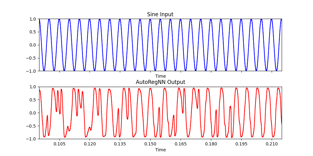
AutoRegNN: 200 Hz sine wave signal #
(
x = {
	var in = SinOsc.ar(200);
	var out = AutoRegNNFilter.ar(in, 1, 12, 8, 1, 0.1, 0.0001);
	[in, out]
}.play
)
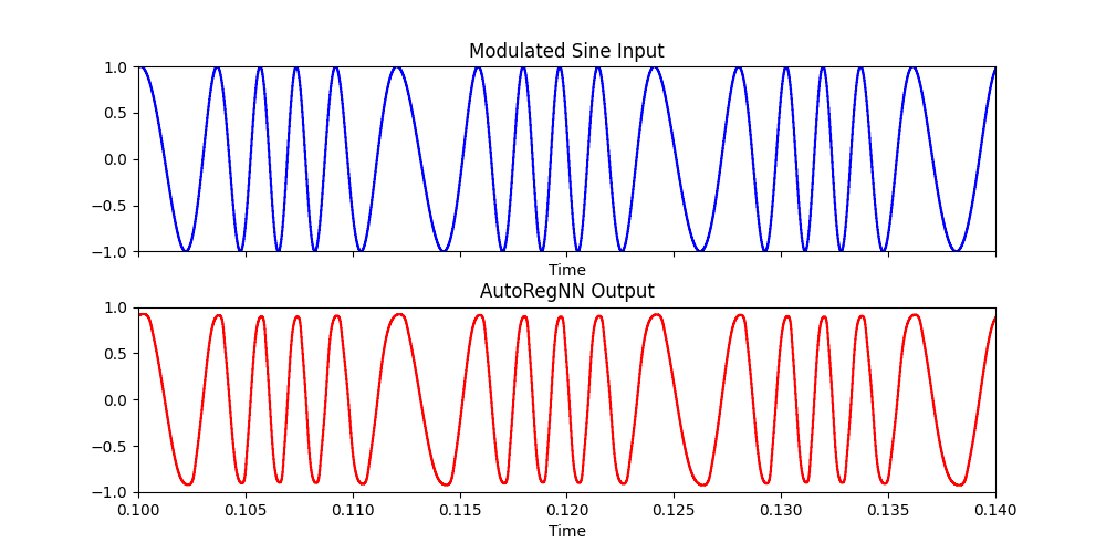
AutoRegNN: Frequency modulated sine wave #
(
x = {
	var in = SinOsc.ar(SinOsc.ar(80).range(220,600));
	var out = AutoRegNNFilter.ar(in, 1, 12, 8, 1, 0.6, 0.01);
	[in, out]
}.play
)
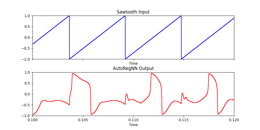
AutoRegNN: 180 Hz sawtooth wave with modulated learning rate #
(
x = {
	var in = LFSaw.ar(180);
	var out = AutoRegNNFilter.ar(in, 1, 12, 10, 1, in.range(0.01,1), 0.00001);
	[in, out]
}.play
)
AutoRegNN: Interpolating between two sets of learned network parameters #
(
{
	var in1 = SinOsc.ar(500);
	var in2 = Pulse.ar(500);
	var out = AutoRegNNFilter2.ar(in1, in2, 0.5, 12, 8, 0.5, 0.001);
	[in1, in2, out]
}.scope
)
AutoRegNN: Multislider Interaction with Model Parameters #
(
Task({
	var size = 8;
	var width = 8;
	var bufferSize = AutoRegNNFilterBuffer.bufferSize(size,width);
	var buf = Buffer.alloc(Server.default, bufferSize);
	var synth;
	var array = FloatArray.fill(bufferSize, {1.0.rand2});
	var w = Window.new("nn", Rect(10,10,bufferSize*20 + 200,500)).front;
	var m = MultiSliderView(w, Rect(10,10,bufferSize*20,480));
	var update = true;
	var lrSlider = EZSlider(w, Rect(bufferSize*20 + 20, 10, 50, 400), "LR",
		ControlSpec(0.0, 0.5, 4, 0.0, 0.1), {arg v; synth.set(\lr, v.value)}, layout: \vert);
	var ridgeSlider = EZSlider(w, Rect(bufferSize*20 + 20 + 50, 10, 50, 400), "Ridge",
		ControlSpec(0.000001, 0.01, 4, 0.0, 0.001), {arg v; synth.set(\ridge, v.value)}, layout: \vert);
	m.size = bufferSize;
	m.value = array.linlin(-1,1,0,1);
	m.elasticMode = 1;
	m.indexThumbSize_(20.0);
	m.action = { arg a;
		buf.sendCollection(a.value.linlin(0,1,-1,1))
	};
	Server.default.sync;
	synth = { arg lr = 0.1, ridge = 0.001;
		var in = SinOsc.ar([40, 51, 82, 99].midicps).sum * 0.2;
		var out = AutoRegNNFilterBuffer.ar(buf, in, 1, size, width, lr, ridge);
		HPF.ar(LeakDC.ar(out),20).dup * 0.7;
	}.play;

	{
		inf.do({
			m.value = array.linlin(-1,1,0,1);
			0.3.wait;
		})
	}.fork(AppClock);


	fork {
		inf.do({
			buf.getToFloatArray(action: { arg a; array = a; });
			0.3.wait;
		});
	};


}, AppClock).play
)
AutoRegNN: Feedback with Three Networks #
(
{
	var in = (WhiteNoise.ar(0.1) * Line.kr(1,0,2)) + LocalIn.ar(1);
	var out1 = AutoRegNNFilter.ar(HPF.ar(in,2).tanh, 1, 12, 10, 1, 0.8, 0.00001);
	var out2 = AutoRegNNFilter.ar(HPF.ar(out1,2), 1, 12, 10, 1, 0.9, 0.00001);
	var out3 = AutoRegNNFilter.ar(HPF.ar(out2,2), 1, 12, 10, 1, 0.8, 0.00001);
	LocalOut.ar(out3+(LPF.ar(out2, 10)));
	HPF.ar(LeakDC.ar(Splay.ar([out1,out2,out3])),20) * 0.6
}.play
)
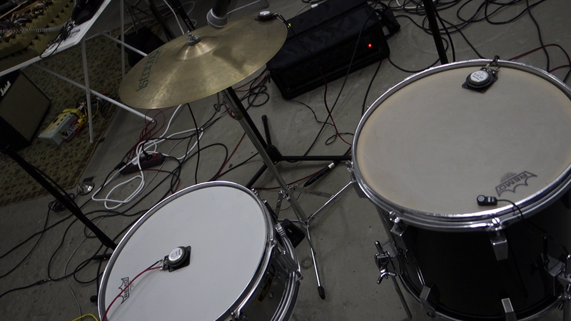
AutoRegNN: Feedback with Percussion Instruments #
Unlearn (forget learning): equations #
\begin{aligned} w_i’(n) = \lambda v_i + s (r - \sqrt{(w_i - u_i)^2 + v_i^2}) w_i \end{aligned}
\begin{aligned} v_i’(n) = - \lambda w_i + \frac {\partial E ( \mathbf{w}_i)}{\partial{w_{i,j}}} + s (r - \sqrt{(w_i - u_i)^2 + v_i^2}) v_i - a v_i \end{aligned}
\begin{aligned} u_i’(n) = w_i - u_i \end{aligned}
Where:
- \(\mathbf{w}_i \) is the vector of all weights for neuron \(i\)
- \(n \) is the current time sample
- \(\lambda \) is the learning rate
- \(s\) is the strength of the limit cycle attractor
- \(r \) is the radius of the limit cycle (typically \(r \ll w_{i,j}\))
- \(a\) acts as a sort of friction to the whole system
- \(u_i\) component of the dynamical system acting as a leaky integrator of the
- \(E (\mathbf{w}_i) \) is the ’lazy neuron’ energy function that has to be minimized:
\begin{aligned} E_i(\mathbf{w}_i) = - \mu f(\sum_{k=1} w_{i,k} x_k(n - d_k)) + \nu g(\sum_{j=1} x_j(n)) \end{aligned}
Where:
- \(f \) is the activation function of the neurons
- \(g \) is a non-linear function of the total energy in the neuron’s vicinity (in the examples below, given the small number of neurons, we take always the energy of the whole network)
- \( \mu \) and \( \nu \) are additional parameters scaling the weight of either part in the minimization of \( E \).
All the following examples have been generated using the henri source code in this repository.
The above repository will also contain a C version of the system using the jack audio library.
Unlearn example 1: self-oscillation #
The network falls into resonant frequencies, which change slowly or suddenly. After initialization, the parameters are left unchanged.
- Size of Network: \( 16 \) neurons
- Activation and energy function: \(tanh \)

-
Delays: random distribution between \( 0 \) to \( 2400 \)
-
\(\lambda ~ 60 \)
-
\( \mu ~ 0.4 \)
-
\( \nu ~ 0.4 \)
-
\(s ~ 0.1\)
-
\(r ~ 0.01\)
-
\(a ~ 0.0\)
See unlearn_16_1.hr henri source code here
Unlearn example 2: self-oscillation decreasing limit cycle strength #
The network self-oscillates. The limit cycle strength is slowly changed during the recording time.
Within noisy patterns, voice like sounds at different frequencies appear and disappear, a sort of confused background chatter. The chatter transforms slowly into a texture of metallic sounds which extend more and more until one equilibrium sound is reached.
-
Size of Network: \( 16 \) neurons
-
Activation and energy function: \(tanh \)
-
Delays: random distribution between \( 0 \) to \( 2400 \)
-
\(\lambda ~ 0.4 \)
-
\( \mu ~ 0.4 \)
-
\( \nu ~ 0.4 \)
-
\(s \) changes from \(160 \) to \(18 \) in the course of the recording
-
\(r ~ 0.01\)
-
\(a ~ 0.0\)
See unlearn_16_1.hr henri source code here
Unlearn example 3: self-oscillation #
Clicky noises, randomly distributed over the network with sudden pauses and isolated fast impulses repetitions
After initialization, the parameters are left unchanged.
- Size of Network: \( 16 \) neurons
- Activation and energy function: “Elevated cosine”
Activation function:

Energy function:

-
Delays: random distribution between \( 0 \) to \( 2400 \)
-
\(\lambda ~ 10.0 \)
-
\( \mu ~ 0.1 \)
-
\( \nu ~ 10.0 \)
-
\(s ~ 0.1 \)
-
\(r ~ 0.02\)
-
\(a ~ 0.5\)
Unlearn example 4: self-oscillation #
“Wind”: very noisy texture, reminding of a recording done holding a microphone into a rainy and windy storm
-
Size of Network: \( 16 \) neurons
-
Activation and energy function: “Elevated cosine” (see above)
-
Delays: random distribution between \( 0 \) to \( 2400 \)
-
\(\lambda ~ 10.0 \)
-
\( \mu ~ 235.0 \)
-
\( \nu ~ 900.0 \)
-
\(s ~ 0.1 \)
-
\(r ~ 0.02\)
-
\(a ~ 0.5\)
Unlearn example 5: self-oscillation #
“Wind / blubber”: noisy texture noise with some bubbling sound. Bubbling get more and more prominent. Oscillation does slowly out.
After initialization, the parameters are left unchanged.
-
Size of Network: \( 16 \) neurons
-
Activation and energy function: “Elevated cosine” (see above)
-
Delays: random distribution between \( 0 \) to \( 2400 \)
-
\(\lambda ~ 28.0 \)
-
\( \mu ~ 0.02 \)
-
\( \nu ~ 900.0 \)
-
\(s ~ 0.1 \)
-
\(r ~ 0.2\)
-
\(a ~ 6.8\)
Unlearn example 6: adapting to a sine #
At the beginning of the recording, one constant sine signal with \( 100 Hz \) frequency is switched on as one of the three inputs of the first neuron.
The network is left adapting until \(1 : 19 \). After that the sine signal is switched off. At the same moment learning is also switched off ( \( \lambda = 0.0 \) referring to the previous equations)
Slowly, after \(1 : 19 \), a clear sine like resonance spreads over the whole network. A remainder of the adaptation.
After initialization, the parameters are left unchanged.
-
Size of Network: \( 16 \) neurons
-
Activation and energy function: \(tanh \)
-
Delays: random distribution between \( 0 \) to \( 4800 \)
-
\(\lambda ~ 1.0 \) then switched off
-
\( \mu ~ 100 \)
-
\( \nu ~ 980 \)
-
\(s ~ 6.5 \)
-
\(r ~ 0.6\)
-
\(a ~ 0.1\)